Estimation of Metal Damage Pattern Using Machine Learning
MIYAZAWA Yuto, CHIBA Ryosuke, OTA Yutaro
MIYAZAWA Yuto : Materials & Structural Engineering Department, Technology Platform Center, Corporate Research & Development Division
CHIBA Ryosuke : Materials & Structural Engineering Department, Technology Platform Center, Corporate Research & Development Division
OTA Yutaro : Doctor of Engineering, Rocket Development Department, Aero Engine, Space & Defense Business Area
Structural materials undergo various types of damage during use, which can lead to deterioration and failure. To prevent failure or recurrence, it is necessary to identify the causes of damage. However, in conventional damage investigations, estimations have been mostly based on the knowledge and experience of evaluators, leading to subjective and unstable results. It is expected to make generalized estimations, that are not dependent on knowledge or experience, by using machine learning image classification methods for microstructure images of damaged materials. This paper presents the prediction results of machine learning model, which accuracy was 89 % by using EBSD (Electron Backscatter Diffraction) images of three types of damaged materials (creep, creep-fatigue, fatigue). This result shows the potential for accurately estimating damage patterns through this method.
1. Introduction
Structural materials undergo various types of damage depending on the service temperature and loading condition, which can lead to deterioration and failure. Particularly, damage in real environments is complicated, as it is often caused by the combined effects of multiple factors such as temperature, average stress, and load amplitude. It is required to analyze the state of materials during maintenance and damage investigation to clarify the causes of damage in order to prevent structural member failures and their recurrence. Generally, the causes of damage to metal materials are estimated based on evaluator’s insights by identifying their states through fracture surface and microstructure observations. Therefore, these estimations lead to subjective and unstable results.
Image classification methods using machine learning are anticipated to effectively solve this problem. It is expected that generalized estimations of damage causes, not reliant on the knowledge and experience of the evaluator, can be achieved by creating a dataset that links images of the microstructures of damaged materials with their respective damage patterns and applying machine learning.
Various types of optical and electronic microscopes are used to evaluate the microstructures of materials. Among them, EBSD (Electron Backscatter Diffraction) analysis is a method for quantitatively analyzing microstructures based on information about local crystal misorientation. Although there are many reports on the correlation between the strain amount and EBSD parameters(1), (2), these EBSD parameters are only applicable for evaluations using average values in visual fields. It is difficult to determine damage patterns only based on the average values of EBSD parameters if the strain amount is equivalent. Additionally, there is an absence of processes, such as evaluating the distribution of EBSD parameters in materials and correlating them with damage patterns.
This paper reports the creation of a model to estimate damage patterns based on the distribution information of EBSD parameters by applying image classification methods to EBSD images using machine learning. In this study, we also analyzed what features in the image the machine learning model focuses on to help clarify the damage mechanism.
2. Test and analysis methods
2.1 Creation of datasets
2.1.1 Material
In this study, Ti-6Al-4V alloy specimens were subjected to three types of damage (creep, creep-fatigue, and fatigue) at room temperature. It is known that the LCF (Low Cycle Fatigue) life of stainless steel and nickel based alloy tends to deteriorate under stress dwell at high temperature(3). This phenomenon is believed to be caused by creep that occurs at high temperature and is known as creep-fatigue. Furthermore, the creep deformation of Ti alloy has also been reported at room temperature(4). Hence, the fatigue life of Ti alloy deteriorates with stress dwell even at room temperature(5). This fatigue with stress dwell at room temperature is known as cold dwell fatigue.
The constant load creep test in this study was conducted with an initial stress of 876 MPa. The fatigue test conditions were a maximum stress of 876 MPa, a stress ratio R = 0, and loading and unloading times of 2 s. In the creep-fatigue test, a stress dwell of 120 s at the maximum stress in the fatigue test was included. These tests were interrupted when the strain reached 4 % in order to maintain an equal amount of strain. The average strain amount obtained from the elongation of the test specimens after the termination of the tests was 4.43 % in the creep test, 4.13 % in the creep-fatigue test, and 4.29 % in the fatigue test.
2.1.2 Acquiring EBSD images
EBSD images of the cross sections parallel to loading direction were acquired from each specimen in six visual fields with an observation magnification of 400 times. The measurement range was 200 × 200 μm. The step size (pixel size) was 0.25 μm. The pixel shape was regular hexagon. Misorientation analysis was applied to EBSD images acquired in this way. Note that only the α phase was used for EBSD analysis in this study though the Ti-6Al-4V alloy has a biphasic structure consisting of the α and β phases. This is because deformation is mainly caused by the α phase and it is difficult to detect the β phase in the grain boundary in EBSD images because the low observation magnification was set to acquire a wide range of data.
In EBSD misorientation analysis, a crystal grain boundary is first defined based on the crystal orientation information for each pixel. Then, the misorientation in each pixel is calculated using various indices. The GROD (Grain Reference Orientation Deviation) and KAM (Kernel Average Misorientation) misorientation analysis indices were used in this study. GROD is an index that indicates the deformation gradient in the grain with reference to the average orientation in each crystal grain. This index is calculated with Equation (1).

Here, θi is the orientation of the i th pixel in each crystal grain, whereas θave is the average orientation, which serves as the reference. On the other hand, KAM is an index that indicates the average misorientation with reference to surrounding pixels. This index is calculated with Equation (2).
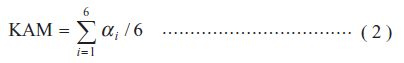
Here, αi is the misorientation between the target pixel and adjacent pixels. That is to say, KAM is the average misorientation between a hexagonal pixel and its six adjacent pixels.
In this study, in addition to the above two analysis methods, we used the grain boundary KAM and intragranular KAM, which are applied analysis methods of KAM. The grain boundary KAM is obtained by extracting measurement points around the grain boundary from the regular KAM. The grain boundary KAM is used when focusing on the misorientation in the grain boundary. On the other hand, the intragranular KAM is obtained by extracting measurement points other than those around the grain boundary. The intragranular KAM is used when focusing on misorientation in the grain. In this study, the area within five pixels of the grain boundary is defined to be around the grain boundary. Hence, measurement points in a 2.5 μm wide area (equivalent to 10 pixels) around the grain boundary were used for the grain boundary KAM, while the remaining measurement points were used for the intragranular KAM.
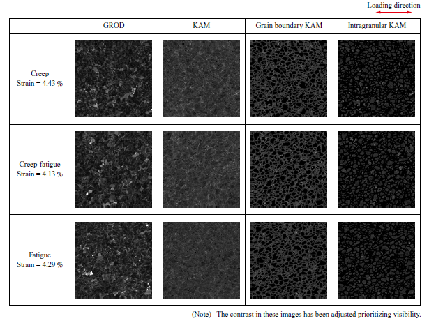
We output EBSD images acquired in the above-mentioned way as grayscale images of 800 (width) × 799 (height) pixels. Figure 1 shows typical visual fields. In each image, brighter pixels indicate larger misorientations. Since the amount of strain in the specimens with each inflicted damage was equivalent, the brightness of the EBSD images was almost the same. Therefore, it was difficult to determine damage patterns by human eye.
2.1.3 Creating datasets from EBSD images
We divided EBSD images of 800 × 799 pixels acquired in six visual fields for each of the three damage pattern types for training and test, and augmented the image data to create datasets for machine learning.
In machine learning, the amount of training data, in which the ground truth (label) for an input is known, is one of the critical factors that directly affect accuracy. Particularly in the materials field, it is difficult to collect a large amount of data in a standardized format due to high experiment costs and complicated manufacturing processes, hindering machine learning. Multiple data augmentation methods have been proposed to increase the number of image data using existing ones to solve this problem in image machine learning. Typical examples include rotation, inversion, translation, cropping, expansion, and reduction.
We employed cropping, rotation, and inversion for data augmentation in this study. Reducing the cropping size increases the number of images generated from an EBSD image. However, the visual field in an image would be narrower, increasing the possibility of events that lead to accuracy degradation. For example, the characteristics of macroscopic damage become difficult to reflect in the data or areas with the characteristics of local damage tend to be excluded from visual fields. Therefore, we compared three sizes of 400 × 400 pixels, 200 × 200 pixels, and 100 × 100 pixels to evaluate the influence of the cropping size. The data augmentation processing generated 72 images that are 400 × 400 pixels, 392 images that are 200 × 200 pixels, and 1 800 images that are 100 × 100 pixels from one EBSD image.
We divided data for training and test from EBSD images before the data augmentation processing. This means that data was divided for training and test before cropped, rotated, or inverted images were mixed in. Specifically, we selected one visual field from the EBSD images of each damage acquired in the six visual fields in advance. Then, we used 72, 392, and 1 800 images of the three damage forms acquired through the data augmentation processing for test and the images in the other five visual fields for training. In this way, the rotated or inverted versions of images used for training are not included in data for test, allowing the prediction accuracy for completely unknown visual fields to be evaluated.
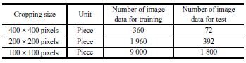
The above processing generated datasets with the number of image data shown in Table 1 for each misorientation analysis method (GROD, KAM, grain boundary KAM, and intragranular KAM) and each damage pattern (creep, creep-fatigue, and fatigue).
2.2 Machine learning method
2.2.1 Network structure
The network structure used for machine learning was ResNet (Residual Networks)(6). This is a type of convolutional neural network. For ResNet, five types with different complexities have been proposed: ResNet-18, 34, 50, 101, and 152. The number of image data handled in this study is approximately 30 000 images at maximum. As this number is smaller than datasets widely known in the image recognition field such as 114 MNIST (Mixed National Institute of Standards and Technology database, 70 000 images) and ImageNet (over 14 million images), we used ResNet-18, which is the simplest network structure. After input images went through multiple convolutional layers, the probability of being classified as each label was calculated with the Softmax function. Cross entropy was used in the loss function that contributes to updating parameters, whereas Top-1 Accuracy is used in validation errors to determine the model to be used. After machine learning using this network, the probability that an image for test was classified as creep, creep-fatigue, or fatigue was calculated with the Softmax function using the model with the minimum validation error. The highest probability among the results was considered to be the prediction result for the image.
2.2.2 Machine learning result evaluation
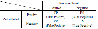
It is necessary to compare the accuracy of acquired machine learning models quantitatively to compare the influence of the misorientation analysis methods and cropping sizes on EBSD. We used three indices (Accuracy, Precision, and Recall) to evaluate the accuracy of machine learning models in this study. These indices are calculated from a confusion matrix. The confusion matrix is a table that summarizes true/false prediction results. Table 2 shows an example of the confusion matrix with two labels. A confusion matrix consists of the same number of rows and columns as that of labels. Each cell contains the corresponding number of image data. For example, the TP cell contains the number of image data for which the actual label and predicted label are both positive whereas the FN cell contains the number of image data for which the actual label is positive but the predicted label is negative.
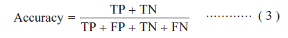
First, Accuracy is an index that indicates the ratio of correctly predicted data to all data. Accuracy is calculated with Equation (3).
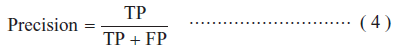
Next, Precision is an index that indicates the ratio of actually positive data to data predicted to be positive. Precision is calculated with Equation (4).
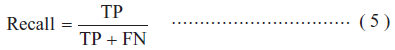
Lastly, Recall is an index that indicates the ratio of data predicted to be positive to actually positive data. Recall is calculated with Equation (5).
Generally, as one of these two indices increases, the other decreases. Which of them is prioritized is determined according to the nature of the problem to be handled.
In this study, since there were three label types (creep, creep-fatigue, and fatigue), the prediction using the machine learning model resulted in a 3 × 3 confusion matrix. Accuracy, and the Precision and Recall for each damage pattern were calculated for this confusion matrix, and these indices were used to compare the influence of the misorientation analysis methods and cropping sizes. We prioritized Recall over Precision in this evaluation because how correctly actual damage patterns are predicted is critical in the subject of this study.
2.3 Analysis of focus areas for machine learning
It was difficult to determine damage patterns by human eye only based on the EBSD images used in this study as described in Subsection 2.1.2. However, if these images can be classified using machine learning, it is suggested that there are differences between EBSD images with different damage patterns that the human eye cannot distinguish, and that these differences are recognized and classified by the machine learning. Therefore, it is assumed that differences in the characteristics of material organization depending on damage patterns can be clarified by visualizing the focus areas for machine learning. Many methods have recently been proposed to visualize what features in the image the machine learning model focuses on during prediction. In this study, we used one of these visualization methods, Grad-CAM (Gradient-weighted Class Activation Mapping)(7), to visualize focus areas.
3. Analysis results and considerations
3.1 Influence of the EBSD analysis methods
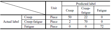
First, we compared differences in the prediction accuracy of damage pattern between the four types of EBSD misorientation analysis methods (GROD, KAM, grain boundary KAM, and intragranular KAM) with a single cropping size of 400 × 400 pixels. Table 3 shows the calculation results of Accuracy, Precision, and Recall gained by applying machine learning using datasets consisting of images acquired with each misorientation analysis method. Both the Precision and Recall of the prediction results for fatigue images are 1.00 with each misorientation analysis method, showing that the prediction accuracy was 100 %. The highest values were achieved for all the indices when intragranular KAM images were used. Table 4 shows the confusion matrix when the intragranular KAM images were used. Although a few errors occurred in distinguishing between creep and creep-fatigue, this suggests a possibility that intragranular KAM images express damage characteristics the best of the four analysis method types considered in this study.
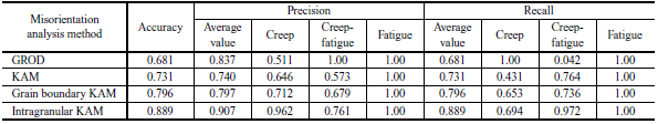
Then, we observed the results gained with the other EBSD analysis methods in detail. First, when GROD images were used, the Recall of creep was as high as 1.00 but that of creep-fatigue was as low as 0.042. This means that most of the creep and creep-fatigue images were predicted as creep. In other words, creep and creep-fatigue were barely differentiated. When KAM images were used, the Recall of creep was below 0.5. That is, more than half of the creep images were predicted to be creep-fatigue, indicating that creep and creep-fatigue were barely differentiated.
Comparison of the results of KAM images, grain boundary KAM images, and intragranular KAM images show that the prediction accuracy of every index is the highest with intragranular KAM, followed by grain boundary KAM and then KAM. Since a grain boundary KAM image and an intragranular KAM image are extracted from specific areas of a regular KAM image, the regular KAM image contains more misorientation information than these two types of images. Nevertheless, the accuracy was higher when grain boundary KAM or intragranular KAM was used. This is probably because materials science information such as grain boundary or intragranular were added to simple coordinate information of pixels with misorientation.
3.2 Influence of the cropping sizes
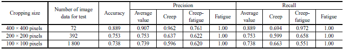
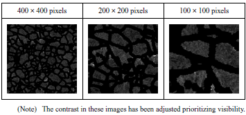
Next, we compared differences in the prediction accuracy between each cropping size. We applied machine learning using datasets of 400 × 400 pixels, 200 × 200 pixels, and 100 × 100 pixels with the intragranular KAM EBSD misorientation analysis method, which showed the highest accuracy in the results in Section 3.1. Table 5 shows the calculation results of the Accuracy, Precision, and Recall of each model. The analysis results of 400 × 400 pixels are the same as those in Tables 3 and 4. Both the Precision and Recall of the prediction results using fatigue images are 1.00 with each cropping size, indicating a prediction accuracy of 100 %. However, regarding the classification of creep and creep-fatigue, the highest accuracy was achieved when images of 400 × 400 pixels were used, and the accuracy dropped as the cropping size became smaller. A possible reason for the degradation of prediction accuracy, despite an increase in the number of image data by five or 25 times, is a decrease in the amount of information per image. Figure 2 shows typical examples of intragranular KAM images after cropping. The number of crystal grains in each visual field significantly varies. Specifically, 400 × 400 pixels, 200 × 200 pixels, and 100 × 100 pixels images contain approximately 150, 40, and 10 grains, respectively. If damage characteristics captured in EBSD images are macroscopic, spanning dozens of crystal grains, it becomes more difficult to identify their entire picture as the cropping size decreases. This probably lowers the prediction accuracy of the model. In contrast, if damage characteristics are concentrated in certain areas, the probability of including those areas in visual fields drops as the cropping size decreases. As a result, a dataset where labels are even given to visual fields with small damage influence is used for training and test. This probably lowers the prediction accuracy. In any case, the result of this consideration shows that the number of image data cannot be increased by reducing the cropping size indefinitely. The most effective method to improve accuracy by increasing the number of image data is likely to acquire additional EBSD images.
3.3 Considerations toward practical application
This section summarizes the model that showed the highest accuracy in the above comparison. The prediction model created by using the dataset generated by cropping intragranular KAM images to 400 × 400 pixels showed the highest accuracy under the conditions considered in this study. Table 4 shows the confusion matrix of the prediction results. Fatigue was predicted with an accuracy of 100 % while Accuracy limited to creep and creep-fatigue was approximately 0.8.
As described above, the method considered in this study showed the potential to determine damage patterns with high accuracy but does not provide determination with an accuracy of 100 %. To actually leverage this method for maintenance or damage investigation, consideration of how to use machine learning models, such as the required accuracy and how to guarantee the validity of prediction results, is required in addition to accuracy improvement and other technical considerations. In addition, discussions on the acquisition method and quality of data input in the machine learning model are necessary, including how to obtain test specimens from actual structures (positions and procedure), how to acquire EBSD images from obtained test specimens, and permissible variations in acquired images.
3.4 Focus area analysis using Grad-CAM
Lastly, we analyzed the focus areas in the intragranular KAM prediction model with a cropping size of 400 × 400 pixels, which showed the highest accuracy in the above comparison, using Grad-CAM. Figure 3 shows the focus area analysis results of creep, creep-fatigue, and fatigue. In Fig. 3, areas closer to red are more focused, whereas those closer to blue are less focused. These are the analysis results of correctly classified images. Figure 3 shows that bright crystal grains in intragranular KAM images, that is, those with large misorientation in the grains, are the main focus areas. The fact that focus areas are located in local areas rather than whole images suggests that the damage pattern may be classified based on the shape of the misorientation distribution occurred in grains as the characteristic, rather than the macroscopic misorientation distribution. Observing focus areas in more detail is expected to lead to the clarification of the damage mechanism in the future.
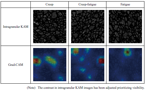
In addition, the size of individual focus areas is equivalent to one to several crystal grains and one image contains few focus areas. This suggests that the prediction accuracy dropped when the cropping size decreased because the probability that visual fields contain areas with remarkable damage characteristics lowered.
4. Conclusion
We applied machine learning using the EBSD images of Ti alloy with the aim of identifying damage patterns that are difficult to determine by human eye. Different types of damage (creep, creep-fatigue, and fatigue) were applied to test specimens at room temperature with equivalent strain amounts, and then EBSD images were acquired.
We compared four EBSD misorientation analysis methods (GROD, KAM, grain boundary KAM, and intragranular KAM), and three image cropping sizes (400 × 400 pixels, 200 × 200 pixels, and 100 × 100 pixels) in data augmentation processing to investigate the influence of these conditions on prediction accuracy. We also analyzed focus areas for machine learning using Grad-CAM and observed what characteristic was focused on in EBSD images during estimation. The conclusion of this study is as follows.
- The model created by selecting 400 × 400 pixels as the cropping size and intragranular KAM as the misorientation analysis method has the highest accuracy among the analysis conditions considered in this study.
- Reducing the cropping size lowers the probability that visual fields contain areas with remarkable damage characteristics, which leads to a lower prediction accuracy. This means that the number of image data cannot be increased indefinitely by reducing the cropping size.
- The method considered in this study shows the potential of determining damage patterns with high accuracy. However, this method does not provide a determination accuracy of 100 %. To put this method into practical application, it is necessary to not only improve the accuracy of the model itself but also figure out how to use the machine learning model and discuss the acquisition method and quality of input data.
- Focus area analysis using Grad-CAM shows that there is a possibility that the shape of misorientation distribution that occurs in crystal grains is used as the characteristic to classify damage patterns. Observing focus areas in detail is expected to lead to the clarification of the damage mechanism in the future.
We will contribute to society in terms of maintenance and disaster control by improving the accuracy of this technology to realize a generalized damage cause estimation that does not rely on the knowledge and experience of evaluator.
REFERENCES
(1) Y. Ota, K. Kubushiro and Y. Yamazaki : Effect of Long Time Stress Dwell on Cold Dwell Fatigue Behavior of Ti-6Al-4V, Journal of the Society of Materials Science, Vol. 69, No. 8, 2020, pp. 599-604 (in Japanese)
(2) K. Kubushiro, Y. Sakakibara and T. Ohtani : Creep Strain Analysis of Austenitic Stainless Steel by SEM/EBSD, Journal of the Society of Materials Science, Vol. 64, No. 2, 2015, pp. 106-112 (in Japanese)
(3) K. Yagi, K. Kubo and C. Tanaka : Effect of Creep Stress on Creep-Fatigue Interaction for SUS 304 Austenitic Steel, Journal of the Society of Materials Science, Vol. 28, No. 308, 1979, pp. 400-406 (in Japanese)
(4) B. C. Odegard and A. W. Thompson:Low Temperature Creep of Ti-6Al-4V,Metallurgical Transactions,Vol. 5,( 1974 ),pp. 1 207-1 213
(5) M. R. Bache:A review of dwell sensitive fatigue in titanium alloys: the role of microstructure, texture and operating conditions,International Journal of Fatigue,Vol. 25,( 2003 ),pp. 1 079-1 087
(6) K. He, X. Zhang, S. Ren and J. Sun:Deep Residual Learning for Image Recognition,Proceedings of the IEEE Conference on Computer Vision and Pattern Recognition,( 2016 ),pp. 770-778
(7)R. R. Selvaraju, M. Cogswell, A. Das, R. Vedantam, D. Parikh and D. Batra:Grad-CAM: Visual Explanations from Deep Networks via Gradient-based Localization,Proceedings of the IEEE Conference on Computer Vision,( 2017 ),pp. 618-626