Method for Improving Operational Efficiency Using Plant Operational Data

　　MOTEGI Yusuke, MATSUDA Kazuma, SUZUKI Yoshitaka, KAWANO Yukihiro

Download PDF

MOTEGI Yusuke : Manager, AI Transformation Promotion Department, Intelligent Information Management Division
MATSUDA Kazuma : Planning and Control Department, Intelligent Information Management Division
SUZUKI Yoshitaka : Manager, AI Transformation Promotion Department, Intelligent Information Management Division
KAWANO Yukihiro : Technical Advisor, Intelligent Information Management Division

At IHI, we are working on leveraging operational data from equipment, and as part of this effort, we are also conducting data analysis using the Mahalanobis Taguchi (MT) method. The conventional MT method is predicated on the assumption that the normal state forms a single group (unit space), and it conducts a one-class classification to distinguish between “normal” and “abnormal” states. However, this approach may lead to false positives or missed detections when the “normal” state changes due to variations in operating modes, ambient temperature, or other environmental factors. To address this issue, a “Dynamic Unit Space MT Method” (hereinafter referred to as “the dynamic MT method”) has been developed, which dynamically selects the appropriate normal data group according to the changing operating environment, thereby achieving high-accuracy classification even for equipment under fluctuating operating conditions. This paper describes the application of the dynamic MT method to improve the operational efficiency of power plants and production facilities, and presents validation results using simulated data.

1. Introduction

It is increasingly required for industrial infrastructures, such as power plants and production facilities, manufactured by IHI, to enhance operational efficiency and reduce environmental impacts and operational costs. In these industrial infrastructures, it is a prerequisite to maintain stable operation of the equipment, even when operational procedures are changed in order to enhance operational efficiency.

There are many control systems that use machine learning to generate operational instructions. Given the prerequisite described above, it is required that these systems provide interpretability to ensure that the equipment continues to operate stably, even when operational parameters are changed. In recent years, the emergence of explainable AI (XAI) has led to the development of solutions to meet these requirements. However, XAI is still under development, which is one of the barriers to introduce it to the aforementioned control systems. On the other hand, there are approaches using highly interpretable physical models and methods to enhance accuracy by integrating physical and statistical models, such as gray-box modeling. However, for facilities like power plants, which are highly complex due to numerous factors such as installation conditions and auxiliary equipment, the cost of accurately developing physical models is high, creating another obstacle to the introduction to the aforementioned control systems. Accordingly, when enhancing the operational efficiency of critical industrial infrastructures, a method is required that provides interpretability for decision-making results and incorporates design expertise as with physical models, while keeping development costs low.

To address this issue, a dynamic Mahalanobis Taguchi (MT) method, developed from the original MT method, was proposed and applied to analyzing plant operational data to improve plant operational efficiency. This paper first discusses the difference between the MT method and the dynamic MT method, and then explains the proposed method. Additionally, this paper presents the verification results of the proposed method using simulated data.

2. MT method and dynamic MT method

2.1 MT method

The MT method is one of the machine learning methods and can effectively perform anomaly diagnosis on multi-dimensional data obtained from equipment with many sensors. It identifies anomalies by using a group of data in the equipment’s normal state, referred to as the “unit space,” as a reference. If the operational data during diagnosis deviates from the unit space, it is considered an anomaly. The MT method measures the degree of deviation using the Mahalanobis distance (hereinafter referred to as “MD value”), which is calculated taking the distribution in the unit space into consideration^{(1), (2)}. A large MD value indicates deviation from the unit space (anomalous state). Each dimension is normalized based on variations within the unit space. Therefore, a meaningful single distance (MD value) can even be calculated from a dataset of sensor values with different unit systems. Figure 1 illustrates the concept of diagnosis using the MT method in the case of two-dimensional data. In Fig. 1, the black circles represent the data that constitute the unit space, while the red cross represents the operational data of the diagnostic target. The blue arrow connecting the black circles and the red cross represents the MD value, and the dashed ellipses represent the contour lines of the MD values.

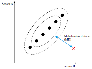
Diagnosis using the MT method consolidates multi-dimensional measurement items into a one-dimension MD value, making it easy to determine whether the operation is normal or anomalous. Additionally, the MT method has the advantage of being able to detect anomalies caused by the breakdown of correlations among multiple measurement items, as well as anomalies with low occurrence since it only learns from the normal state.

On the other hand, the MT method may lead to false detections or missed detections when the normal state itself changes due to the equipment’s operating environment, such as external conditions and operational parameters. It is possible to come up with a method of addressing changes in normal states due to operating environment by pre-assigning a unit space to each cluster of normal states that vary according to the operating environment and representing all normal states across multiple unit spaces. However, it is difficult to practically apply such a method in cases where normal states change continuously or where a large number of clusters are needed to represent the normal states. To address these challenges, a dynamic MT method, as explained in Section 2.2, was proposed.

2.2 Dynamic MT method

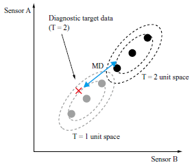
In the dynamic MT method, data on normal states under various operating environments are prepared in advance, and for each diagnosis, only data from the vicinity of the equipment’s operating environment are extracted to generate a unit space. In this paper, the unit space generated at each time point is referred to as a dynamic unit space. Figure 2 illustrates a conceptual diagram of a dynamic unit space. As shown in Fig. 2, when diagnosing the operational data at time T = 2, represented by a red cross the dynamic unit space generated at time T = 2 is used to calculate the MD value.

Unlike the conventional MT method, which uses a pre-fixed unit space constituent data group, the dynamic MT method can arrive at an appropriate diagnosis even when the normal state changes, as a unit space is generated from the data group in the vicinity of the operating environment each time a diagnosis is performed^(3)–(6).

In selecting the data group used to generate a dynamic unit space, the dynamic MT method uses items related to the operating environment of the target equipment, such as ambient temperature, atmospheric pressure, and set output, rather than the items constituting the unit space, such as sensors A and B in Fig. 2. The selection conditions (operating environment conditions) are set based on the knowledge of how the target equipment was designed, including the items to be used and the range of values considered as data in the vicinity of the operating environment.

Due to the clear process of generating dynamic unit spaces and performing diagnoses, the dynamic MT method provides high interpretability of the determination results, even for complex equipment with changing operating environments.

3. Enhancing operational efficiency with the dynamic MT method

3.1 Method of defining dynamic unit spaces

We are proposing a method of enhancing operational efficiency by using operational data from plants. Since it is necessary to consider the influence of the operating environments of plants, as is the case with anomaly diagnosis, the concept of dynamic unit spaces, as explained in Chapter 2, is applied in this method.

As an indicator of operational efficiency, thermal efficiency is used in this paper as an example. This method includes a preparatory phase, in which a target for the extent of improvement in thermal efficiency is set, and a regular diagnostic phase, in which measures to improve thermal efficiency are identified at each time of diagnosis. Table 1 shows the plant environmental conditions, diagnostic target items, and purposes of processing for the preparatory phase and the diagnostic phase.

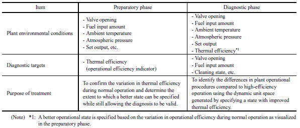
The diagnostic target items that constitute the dynamic unit space in the diagnostic phase represent internal states of the plant in the case of anomaly diagnosis, but in the case of improving operational efficiency, the target items related to plant operational parameters, such as valve opening, fuel input amount, and cleaning to improve thermal efficiency, are used. As in the case of anomaly diagnosis, the plant environmental conditions are set based on the knowledge of how the target equipment was designed, and include external environmental factors and operational conditions that affect the plant’s operation. However, thermal efficiency has been added as a target item and the range considered to be the vicinity of the operating environment is set to be higher than the thermal efficiency at the time of diagnosis. This range serves as the target value for the extent of improvement in thermal efficiency. Since extent of improvement has a the-larger-the-better characteristic, it is basically preferable for it to be as large as possible. However, if the value is set too high, beyond the range present in the training dataset, the unit space cannot be generated. Therefore, it is necessary to appropriately set the value range based on the distribution of the training dataset. Additionally, the value range must be set in consideration of the effects of changes in the operating environment. Therefore, the preparatory phase is established to preliminarily grasp the typical range of distribution of thermal efficiency values under similar operating environments.

In the preparatory phase, the plant environmental conditions, excluding thermal efficiency, are the same as those in the diagnostic phase. In this phase, only thermal efficiency serves as the diagnostic target item that constitutes the dynamic unit space. By examining thermal efficiency values within the dynamic unit space, the possible range of thermal efficiency under similar operating environmental conditions can be identified. Based on this range, an appropriate target for improvement can be determined.

In the diagnostic phase, thermal efficiency is added to the operating environmental conditions, and the extent of its improvement is set in the vicinity of the operating environment. By setting the extent in this way, it becomes possible to extract, as a dynamic unit space, a group of data under operating environments similar to those at the time of diagnosis and with higher thermal efficiency than at that time.

3.2 Selecting target period for operational efficiency improvement using MD values

Figure 3 illustrates the vector quantities representing the improvement in thermal efficiency. In Fig. 3, the XY coordinates represent the operational parameters’ values, and the Z axis shows the thermal efficiency value. The blue areas represent the entire training dataset, the black dot represents the data at the time of diagnosis, and the green areas represent the data within the extracted dynamic unit space. As can be seen from the fact that the Z-axis values of the green areas are higher than that of the black dot, the green areas represent data with higher thermal efficiency than at the time of diagnosis under similar operating environments. That is, the blue arrow represents the correction amount in operational parameters required to improve thermal efficiency from the time of diagnosis.

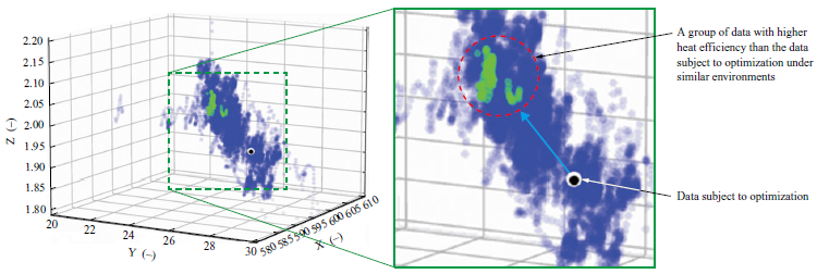
However, since the number of plant operational parameters is extremely large, it is rarely possible to represent them in a low-dimensional space as shown in Fig. 3, making it difficult to identify operational regions where thermal efficiency can be effectively improved. Therefore, MD values calculated for each diagnostic target data using the MT method are utilized.

An operational region with a high MD value indicates that, under similar operating conditions, there exists a state with better thermal efficiency and that there are significant differences in the operational parameters’ values. Therefore, such an operational region is considered to have a high potential for improving thermal efficiency through correction of the operational parameters’ values. Conversely, an operational region with a low MD value corresponds to a region in which there are few differences in operational procedure variables. In such cases, changes in thermal efficiency are presumed to result from external factors such as ambient temperature or weather conditions. Therefore, this type of operational region is considered unlikely to benefit from efficiency improvements through correcting the operational parameters’ values.

Since the MD value is a one-dimensional metric, extracting data with high MD values from the data within the dynamic unit space makes it relatively easy to identify periods during which thermal efficiency can be improved.

3.3 Checking the operational parameters to be corrected based on their degree of contribution

Using the method presented in Section 3.2 enables certain periods during which thermal efficiency can be improved to be detected solely on the basis of the MD value. However, because the MD value aggregates multidimensional information into a single dimension, it alone cannot reveal which operational parameters contribute most to the differences in thermal efficiency.

To address this issue, we decided to use the contribution degree provided by the MT method. Because the contribution degree indicates how strongly each item influences the MD value, examining the operational parameters with high contribution degrees during periods when the MD value is elevated makes it easy to identify the operational parameters most likely to affect thermal efficiency. Figure 4 illustrates an example of extracting operational parameters subject to improvement. In the high-MD operational region from 874 to 886 shown in Fig. 4-(a), the operational parameter labeled MD Contribution Degree_24, represented by a green line and showing the highest contribution in Fig. 4-(b), is judged the most likely to improve thermal efficiency.

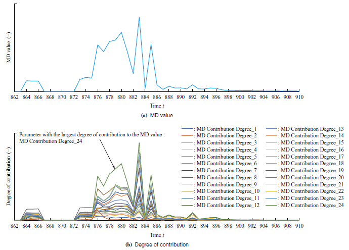
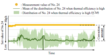
Figure 5 shows the visualized correction amounts for the operational parameter subject to improvement. The figure shows a time-series comparison: the distribution within the dynamic unit space (mean ± 3σ) of the high-contribution operational parameter identified in Fig. 4 is shaded in green, while the measurement at the time of diagnosis is highlighted in yellow. As Fig. 5 shows, the value range of the displayed operational parameter differs markedly between the operational region in the training phase when thermal efficiency reached its target and that in the diagnostic phase. Thus, revisiting this parameter’s setpoint is therefore expected to improve operational efficiency.

When selecting a target period and a target operating parameter to improve operational efficiency, it is preferable to select the operational parameter whose degree of contribution remains consistently high within the operational region where the MD value is also continuously high over time. In such an operational region, a plant is presumed to be nearly steady state. Therefore, even if the diagnostic target item constituting the dynamic unit space is limited to the operational parameter’s value at each time as described above, the diagnostic results are unlikely to be significantly affected.

In contrast, a plant’s internal state is generally affected not only by operational parameters’ values at that time, but also by past operational amounts. Therefore, when a plant is in a transient state, due consideration is required to add the past operational amounts affecting the internal state to the diagnostic target items constituting the dynamic unit space.

A key advantage of this method is that both the recommended correction for each operational parameter and the corresponding expected efficiency gain are derived from real data in the training dataset, ensuring that the proposed improvements are highly feasible in practice.

4. Verification

4.1 Target data

The method proposed in Chapter 3 was verified using simulated data. For this study, we used an open dataset⁽⁷⁾ containing time-series operating data from a supercritical-pressure boiler.

The dataset comprises 115 key items that describe the plant’s internal state, operating environment, and operational parameters, including: GENERATOR MW (generator output); TOTAL COAL FLOW BEF CAL CORR (total coal flow); TOTAL AIR FLOW (t/h) (total air flow rate in t/h); AA (L) CRNR 1 AA DMPR FB (damper-opening feedback); and many others. The dataset contains 17,280 rows (observation points), all recorded while the equipment was operating under normal conditions. Of these, 15,840 rows were used as training data (to extract the dynamic unit space), and the remaining 1,440 rows served as verification data for improving operational efficiency. The verification dataset was created without random sampling; instead, the data were split so that the original temporal continuity was preserved.

4.2 Calculation of operational efficiency indicator

In boilers, most of the thermal loss stems from flue-gas discharge. Calculating this loss normally requires the exhaust gas specific heat, but the necessary information is missing from the present open dataset. Therefore, for simplicity, we adopt Equation (1) as the operational-efficiency indicator (hereinafter referred to as “G_C_RATIO”).

4.3 Setting conditions for dynamic MT method

Based on our boiler design expertise, we selected the items listed in Table 2 as the operating environmental conditions used to identify data points in the vicinity of the operating environment.

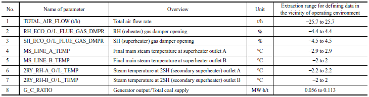
Among the operational environmental conditions, to extract the data in the vicinity of the plant’s operating environment, the extraction range of Items Nos. 1 to 7 was set applying the same ± tolerance on both sides. This extraction range was determined from a design standpoint.

In contrast, as mentioned in Section 3.1, the extraction range of G_C_RATIO for No. 8 was set to + 0.056 or more and + 0.113 or less with respect to the verification data used only for the positive side based on the distribution area observed under similar operating environments confirmed in the preparatory phase. In other words, to generate the dynamic unit space, we extracted from the training data group only records whose operating conditions were similar to those of the verification data and whose G_C_RATIO was at least 0.056 MW·h/t of coal. We then compared this space with the verification data.

4.4 Method for setting extraction range of operation efficiency indicator

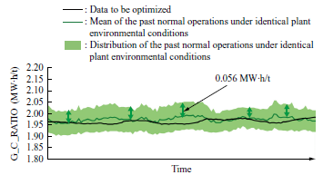
The extraction range of G_C_RATIO mentioned above was set based on the distribution area of G_C_RATIO obtained in the preparatory phase. Figure 6 illustrates the improvement range setting for the operational indicator. The distribution range in Fig. 6 represents the standard deviation (1σ). Given that the verification data are assumed to follow a normal distribution like that of the training data, because both datasets were obtained under similar operating environmental conditions, the improvement range for the operational efficiency indicator was set to +1σ to +2σ (0.056 to 0.113), assuming it is achievable at the level where actual data exist.

4.5 Generation of dynamic unit space toward operational efficiency improvement

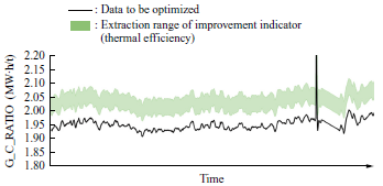
Figure 7 shows the distribution of the extracted data group with high thermal efficiency, and Fig. 8 shows the correction amounts of the operational control values. In Fig. 7, the vertical axis represents G_C_RATIO, and the horizontal axis represents time. The black line represents the verification data values, and the green shaded area indicates the extraction range of the operational efficiency indicator (G_C_RATIO).

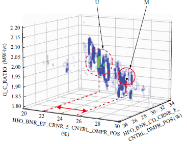
Like Fig. 3, Fig. 8 is displayed in three dimensions to represent G_C_RATIO among other operational parameters’ values, and it illustrates an extraction result at a specific point in time, rather than as a time-series data. Thus, a correction value was obtained by setting the improvement target to an operational parameter that has a large MD value between the measurement point M, represented by the black dot to indicate the verification data, and the dynamic unit space U, represented by the green shaded area, and that has a high degree of contribution as indicated by the red arrow, which shows the direction with the largest deviation among the dimensions constituting the MD value in Fig. 8.

In this case, the improvement target selected was HFO_BNR_EF_CRNR_5_CNTRL_DMPR_POS (control-damper position) as it had the highest degree of contribution. Although Fig. 8 visualizes only instantaneous values at a specific point in time, we also calculated the average difference between the mean of the dynamic unit space U over the entire continuous period selected for improvement and the measurement point M. That analysis indicated that shifting the control-damper position by −2.4% could be expected to improve G_C_RATIO.

Naturally, there are cases where it is preferable to adjust several operational parameters rather than just one. By using the degree of contribution in the MT method, it is thought possible to identify and extract the multiple appropriate operational parameters even in such situations.

4.6 Calculating expected value for operational efficiency improvement

We re-extracted data that shared similar operating environments and had HFO_BNR_EF_CRNR_5_CNTRL_DMPR_POS at −2.4% from the training dataset. We then compared those records to see how G_C_RATIO changed. Figure 9 illustrates the thermal efficiency improvement range after the correction amount has been applied. In Fig. 9-(a), the vertical axis shows the G_C_RATIO values and the horizontal axis shows operating time. The black line traces the time-series values of the verification data, while the green shaded area depicts the time-series distribution (± 1σ) of the data extracted from the training data. Fig. 9-(b) plots G_C_RATIO on the vertical axis and HFO_BNR_EF_CRNR_5_CNTRL_DMPR_POS on the horizontal axis. Like Fig. 8, it is a scatter plot at a single point in time.

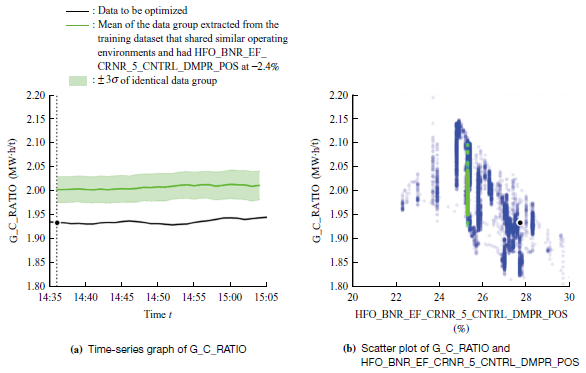
Because the data are time-series, the adjustment will not lead to a uniform improvement in G_C_RATIO at every moment; nonetheless, it is expected to raise the mean from roughly 1.93 to 2.01 MW·h/t. This represents an efficiency gain of approximately 3.7%. In this dataset, because the training and verification datasets showed no significant differences in the boiler’s operating environment or internal states, this improvement measure appears to be practically feasible.

5. Conclusion

5.1 Summary

We have proposed applying the dynamic MT method to plant operating data in order to identify, with interpretable reasoning for the determination of correction, the operational regions in which efficiency can be improved and the specific operational parameters that should be adjusted along with their recommended correction amounts, even for plants whose complex internal states fluctuate with changing operating conditions. By applying the proposed method to simulated data and analyzing the results, we confirmed its effectiveness, estimating an improvement in thermal efficiency of approximately 3.7%.

5.2 Challenges

Since the proposed method uses operational parameters as the diagnostic items constituting a unit space, the extracted dynamic unit space may constitute some clusters in those plants where operational parameters differ even under identical operating environments. A key challenge is to accurately identify the operating regions where improvement can reasonably be expected even in such cases. Additionally, for plants in which past operation histories greatly influence changes in internal states, a remaining challenge is to handle not only steady state but also transient states in which the internal states vary markedly. Moreover, the proposed method has yet to elucidate the causal relation between changes in operational parameters’ values and improvements in thermal efficiency. Therefore, establishing and explaining this causality remains an outstanding challenge.

5.3 Future Development

We are presently applying the proposed method to an operating plant and will demonstrate that it effectively improves thermal efficiency in actual operation. Additionally, although this paper has focused on plants’ thermal efficiency, the proposed method can also be applied to other operational efficiency indicators such as carbon dioxide emission reduction rate, power consumption reduction rate, and product yield rate. Going forward, we will extend this method across a wide range of IHI products to boost their operating efficiency and, in turn, enhance customer value over the entire product life cycle.

　　　　 　　　　 　　　　 　　　　 　　　　 　　　　 　　　　 　　　　 　　　　 　　　　 　　 　 　 　 　 　 　 　 　 　 　 　 　 　 　 　 　 　 　 　 　 　 　 　 　 　 　 　 　 　 　 　 　 　 　 　 　 　 　 　 　 　 　 　 　 　 　 　 　 　 　 　 　 　 　 　 　 　 　 　 　 　 　 　 　 　 　 　 　 　 　 　 　

Vol.58 No.2

REFERENCES

(1) H. Yano : Collected Papers of Genichi Taguchi, Vol. 4, Japanese Standards Association, 2012 (in Japanese)
(2) S. Sodekoda, M. Kimura, Y Suzuki and C. Kondo : Development of Preventive Maintenance Technique using Data Analysis, Journal of IHI Technologies, Vol. 54, No. 2, 2014 (in Japanese)
(3) Y. Motegi, S. Sodekoda and Y. Kono : Accuracy Improvement of Plant Diagnosis by Optimizing Unit Space, The 48th Symposium on Reliability and Maintainability, 2018 (in Japanese)
(4) Y. Motegi : Improving the Accuracy of Anomaly Diagnosis for Mechanical Equipment and Plants by Dynamically Generating Unit Spaces, Research Presentations at the 27th Robust Quality Engineering Society Annual Meeting, 2019 (in Japanese)
(5) H. Nagashima, Y. Hasegawa, Y. Motegi and Y. Kono : Development of Anomaly Diagnostic Technology using Machine Learning, Journal of IHI Technologies, Vol. 60, No. 1, 2020 (in Japanese)
(6) Y. Motegi : Anomaly Diagnosis for Industrial Equipment Using the MT Method with Dynamic Unit Spaces Applied, Research Presentations at the 29th Annual Meeting of Robust Quality Engineering Society, 2021 (in Japanese)
(7) kaggle : About Dataset, Power Plant Optimization Problem, https://www.kaggle.com/datasets/deepakburi062/power-plant-optimization-problem, accessed 2024-11-01